
7. Layout optimization
After the Energy Map and Constraints Map are defined, optimizations of n=1..N layouts can be performed. The pre-existing constraints of IEC exclusion areas, park areas and other ara constraints are already defined in the Constraints Map module.
In the layout optimization module, each layout, n can be constrained with:
- Minimum distance constraints
- Elliptic distance constraints
- Effective turbulence constraints, or a combination thereof.
While the IEC exclusion areas can are straightforward to include, the distance constrants are what makes the layout optimization a difficult optimization problem. Where you place one turbine potentially affects where you can place the other turbines du to the interdependencies of wake losses and wake induced turbulence.
The figure below shows the layout module
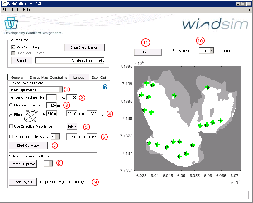
layout optimization module
7.1 Optimization algorithms
Three alternatives for optimization can be selected, see (1) on the figure: Basic Optimizer, WFD cloud optimiziation and WFD local optimiziation
Basic optimization algorithm is a heuristic algorithm based on simulated annealing, and provides near-optimal solutions. Methods such as simulated annealing, genetic algorithms and similar trial-and error algorithms can find good results, but are slow compared to more formal optimziation techniques, and does not provide information about the quality of the solution.
The basic optimization algorithm is default and does not require extra licenses for use.
WFD cloud optimization * is a highly specialized optimization routine based on formal operations research methods, and solved by state-of-the-art optimization solvers. The WFD optimziation algorithm can guarantee global optimum for layout optimization problem, subject to minimum distance, elliptic distance and wake induced turbulence constraints.
To our knowledge this is the only optimizer available that guarantees global optimum with the above mentioned distance constraints. Wake losses are however not included in the optimization, but we argue that the distances required for effective turbulence constraints dominate the importance of wake losses, see article xx
WFD cloud optimization is a cloud service, and can be called from within ParkOptimizer. The cloud optimziation upload the problem to the WFD server (hosted on google compute engine), that runs the optimization algorithm with state-of-the-art solvers and return the results to parkoptimizer.
WFD cloud optimization can be purchased on a per use basis, or with a periodic license. Contact klaus@windfarmdesigns.com for more information
* Requires internet access
WFD local optimization is the same optimization algorithm as WFD cloud optimization but deployed as an executable running on the client’s local server. This alternative is intended for larger organisations for in-house use, and requires additional licenses.
Terrain inclination is not a part of the IEC standard, but is useful for practical purposes. Terrain inclination are areas unsuitable for turbine placements because of steep slopes and/or steep road access . These constraints are not absolute, and can be remediated by proper civil works at some increased costs. Moreover, steep terrain causes flow inclinations as well (see next section), and these constraints often overlap.
At an early stage of the project development, it is useful to get an indicator of the problem with terrain fro screening of sites, and for initial layouts and derived energy yield estimates.
Terrain inclination is derived from the WindSim input files, \dtm\view_inclination.scl
7.2 Optimization settings
Number of turbines
A special feature of ParkOptimizer compared to other wind farm tools, is that you can optimize for a range of layouts, n=1..N. If the layout size is not fixed, layout size can have as significant impact on the profitability of the project, and on the project risk, as we will explain in the economy module. Select the Number of turbines by entering Min and Max values, see (2) in the above figure.
Distance constraints
You can specify either Minimum distance (see 3 in figure) or Elliptic distance with parameters a,b and deg, where a is the diameter in [m] along the major axis, b is the diameter in [m] along the minor axis and deg is the orientation of the ellipse major axis measured in [deg].
The elliptic distance constraint (see 4 in the figure) has become a proxy for wake losses and wake induced turbulence, as these are more pronounced in the prevailing wind direction. A typical choice of paramterers are a=5 RD, b=3 RD where RD = rotor diameter. The orientation depends on the wind rose.
7.3 Effective turbulence
Effective turbulence can be specified by checking Use Effective Turbulence (see 5 in figure) and editing the Setup as follows:
- Effective turbulence is calculated based on the .tws mast file, also used in the IEC constraints module, see (1) on figure below.
- If a measurement mast is to be used for turbulence calculations, check (2) on the figure below
- Set the the Wöhler coefficient in (3) and check the terrain complexity index (4) if needed. See also discussion in section 6.4 Turbulence
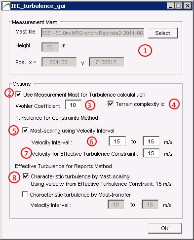
Turbulence GUI
Characteristic turbulence should be checked for a range of wind speed intervals, ranging from 


At this moment, the velocity range to check for the effective turbulence is considered in the IEC exclusion area map (i.e. the ambient effective turbulence) (point 6 on figure) whereas for the wake induced effective turbulence, the constraint is only checked for one wind speed interval (see (7) on figure).
Method of turbulence extrapolation
The default method for turbulence extrapolation , is by scaling the map with the mast, where the wind map is adjusted by the ratio of the measured wind speed and the simulated wind speed at the mast point and sector, extrapolated to each map point, see
An alternative method, more precise but also more time consuming, is to also scale mast according to various wind speed bins (see (8) on figure).
7.4 Wake losses
Wake losses
Wake loss calculations are preferably applied after a layout satisfying the minimum distances are created. For wake loss calculations, N.O Jensens model is applied:
 = dV(s) = v_0 \cdot (1-\sqrt{1-C_t(v_0)}) \cdot (\frac{D}{D+2kx})^2")
where x is the down stream distance of the rotor with diameter R, and \alpha is the wake decay coefficient, also denoted as k (see (6) in figure 7.1 layout optimization module)
The parameters for the wake model, rotor diamter D, wake decay coeffefficient k=0.075 (default) and the number of iterations are defined by the user (see (6) in figure 7.1 layout optimization module), and indicates how many attempts the simulated annealing algorithm will check to find better turbine placements.
Start optimizer
We recommend to not use wake loss calculations for the optimization, the wake loss adjustments can be run later to adjust a layout where the distance constraints are satisfied.
To start the optimizer, press Start Optimizer button (see (7) on figure 7.1 )
 Wake loss adjustment[/caption]
7.5 Improve layouts
Improve layouts
Once a layout satisfying the distance constraints are establishe, we recommend to run optimized layouts using with wake effects, (see (8) on figure 7.1 ), where the number in the dropdown menu defines the number of times the simulated annealing process is run for wake effect adjustments. For each run , there will be a new folder with layout files.
Performing wake effect adjustment will modify the layouts and write the files to Results_Directory\OPT_OUT\wake_effect_adjusted. The following method is employed for each layout :
Let PC and Ct be the turbine specific power-curve and thrust-coefficient, as defined in the Turbine File ( set in the Energy Map module) and let A(s), k(s), f(s) be the Weibull parameters for sector s of points in the Wind Resource file.
The energy production at each point , incorporating wake effects, is calculated as follows
- A dV – change in wind speed due to wake – matrix is constructed for each sector accounting for each turbine position p. Let
at a turbine position p ( we are using the A parameter as an approximation to the average wind speed ).
Then dV for sector s , dV(s), due to turbine at position p is,
where
and D = Rotor Diameter, and where the calculation is done for values of x within a cone downwind of the turbine position p inside +/- 15 deg (if the data-set has 12 sectors; correspondingly less for 16 and 24 sectors) of the sector s direction and radius
. If a point is affected by more than 1 wake, the
values are added.
- The energy at each point , incorporating wake effects, is the sum over the sectors s of
, over
where wbl is the Weibull probability distribution function
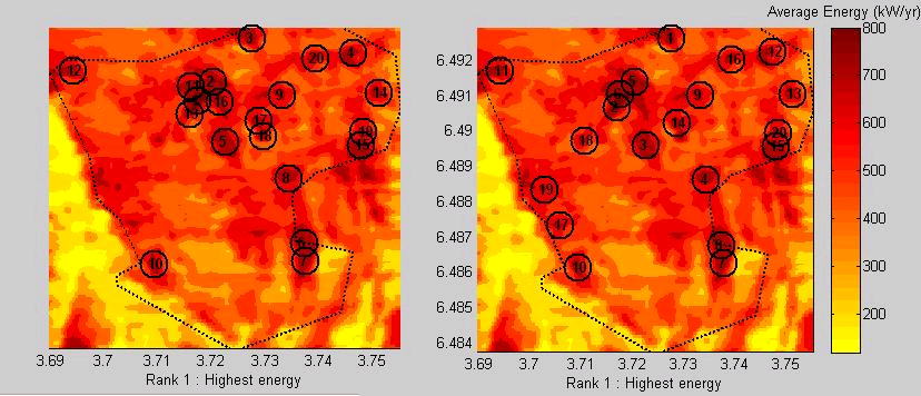
This wake effect adjusted energy map is then used to move turbines so that the total energy production will be higher. The optimization method is based on Simulated Annealing.
The figure below illustrates the wake adjustment. Press the Figure button (see (11) in above figure) in the gui to produce the figures ( note that the circles are markers, and do not indicate distance ). The layout size can be chosend from the nearby dropdown menu (see 10 on the above figure)
Open layouts
All optimization results are stored in the folder OPT_OUT, containing
Layout0001.txt, ….
Layout0002.txt,…
Layout00NN.txt
in the form of text files with turbine coordinates, as well as an energy_curve.txt file containing the corresponding energy yield for each layout size.
Existing layouts can be downloaded into the project.