<<< 2.0.0 Morbi et sodales To overview >>>

6. IEC exclusion areas

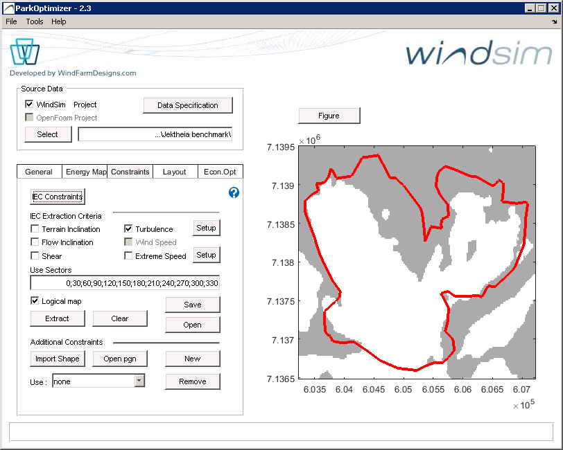
IEC exclusion areas are represented by the gray areas in the figure below. The white areas show valid turbine positions. IEC exclusion areas can be calculated as a combination of type and sectors. If only one sector and one constraint type is involved, a map of absolute values can be displayed. Otherwise, the constraints and sectors are superimposed as logical maps.

IEC Exclusion areas

Press the IEC Constraints button to view/edit the constraint limits, and press the Extract button after selecting one or several of the following IEC Constraints, to generate the Constraints Map . By IEC constraints and exlusion areas, we refer to the IEC 61400-1 3rd ed. standard (2005), plus its amendment (2010). The standard defines design requirements for wind turbines, including ranges of wind quality aspects that the turbines should tolerate. The ones considered in ParkOptimizer are:

Terrain Inclination (not part of the IEC standard). Data is retrieved from view_inclination.scl of WindSim input files.
Flow Inclination. Calculation based on windspeed files of WindSim input files.
Shear. Calculation based on wind speed files of WindSim input files in three heights corresponding to hub height and the +/- heights defined by shear deviation
Turbulence intensity
Extreme wind

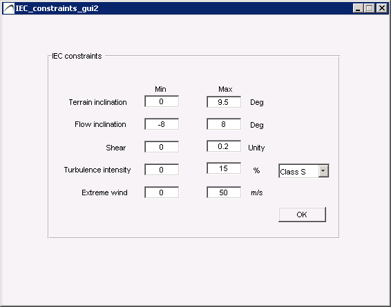
IEC constraints definitions

6.1 Terrain inclination

Terrain inclination is not a part of the IEC standard, but is useful for practical purposes. Terrain inclination are areas unsuitable for turbine placements because of steep slopes and/or steep road access . These constraints are not absolute, and can be remediated by proper civil works at some increased costs. Moreover, steep terrain causes flow inclinations as well (see next section), and these constraints often overlap.

At an early stage of the project development, it is useful to get an indicator of the problem with terrain fro screening of sites, and for initial layouts and derived energy yield estimates.

Terrain inclination is derived from the WindSim input files, \dtm\view_inclination.scl

6.2 Flow inclination

Flow inclination uses the uses vertical and horisontal wind speeds from Input files to calculate the flow inclination. The flow inclination is calculated as the maximum inclination over the sectors s at each location (x,y). If the maximum inclination exceeds the constraints defined in IEC constraints definitions (see figure above) then the location is an exclusion and presented as a gray point on the exclusion map.

6.3 Shear

The shear calculation uses wind speed Input Files, at heights defined with the Hight Definition button. In addition, the Wind Resource file selected in the Energy Map tab will provide the frequency of each sector : f(s).
Let $v_1, v_2 and v_3$ be the wind speed values corresponding to heights $h_1= Simulation Height+Shear Deviation$ , $h_2=Simulation Height$ and $h_3=Simulation Height -Shear Deviation$ respectively. Further, let s be each of the sectors listed in the Use Sectors box of Constraints Map tab. Then the shear coefficient $\alpha(s)$ for sector s , at each point is the (Least Squares) solution of the equations

$v_1(s)/v_2(s) = (h_1/h_2)^{\alpha(s)}$
$v_3(s)/v_2(s) = (h_3/h_2)^{\alpha(s)}$

The shear coefficient $\alpha$ is then the sum over the Use Sectors $\sum_s \alpha(s)\cdot f(s)$ .

Note that if the Wind Resource file is not defined, the shear coefficient will be set to the maximum over the sectors of $\alpha(s)$ .

6.4 Turbulence

Turbulence is calculated from the turbulence intensity files of Input Files at the Simulation Hight, scaled according to a tws measurement file (if defined, in which case a turbulence intensity at the measurement height is also required). The Wind Resource file selected in the Energy Map tab provides frequency distribution of the sectors.

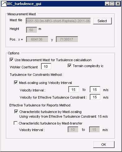
Turbulence GUI

Select the tws measurement file by pressing turbulence Setup:

First, select a .tws wind measurement file containing 10-min wind speed time series [m/s] and its associated standard deviations sd [m/s] within the 10-min time wind speed interval. The .tws file also contains information about its location and measurement height.

The exclusion areas are computed as Ambient effective turbulence intensity, defined as:

(1) $I_a/V_{hub} = {1\over V_{hub}} \cdot[\sum_s \sigma_c(s,V_{hub})^m f(s)]^{1/m}$

where

-m is the Wöhler exponent (default value is 10 for turbine blades (composite), 5 for tower (steel) )

– $\sigma_c$ the characteristic turbulence latex]\sigma_c =1.28\sigma_\sigma[/latex], i.e. the 90th percentile of the turbulence standard deviation

– $V_{hub}$ is wind speed at hub height.

Method 1: Turbulence intensity map from WindSim is used directly.

To use this method, uncheck “Use Measurement Mast for Turbulence calculation”. The Wöhler coefficient and terrain complexity check still applies to the results. This method is recommended when there is no mast data available, or the mast data is of poor quality.

According to WindSim documentation, $TI = {100}\cdot {{\sqrt{4/3 KE}}\over{\sqrt{UCRT^2+VCRT^2}}}$ (%) for each sector s

the resulting $TI(s)=\sigma_T(s,V_{hub})$ is then used to calculate the the Ambient effective turbulence (see equation (1) above)

Method 2: Turbulence intensity map from WindSim is scaled with mast data.

To use this method, check “Use Measurement Mast for Turbulence calculation”. The Wöhler coefficient and terrain complexity check. This method is recommended when there is no mast data available, or the mast data is of poor quality.

The turbulence at each point ( assuming a measurement file is used ) is calculated as follows. For each sector s, let TI(s) be the turbulence intensity at the Simulation Height, $TI_{meas}(s)$ the turbulence intensity from the measurement file (at the measurement height), $TI_{ws}(s)$ the WindSim turbulence intensity at the same coordinate and height as $TI_{meas}$ , and $f(s)$ the sector frequency from the Wind Resource file, then the scaled turbulence intensity $TI_{scaled}(s)$ is the frequency weighted sum over sectors s in Use Sectors

$TI_{scaled}(s) = {TI(s) \cdot f(s) \cdot {TI_{meas}(s)} \over TI_{ws}(s)}$

The resulting $TI_{scaled}(s)$ is then used to calculate

If the wind resource file is not defined, the turbulence at each point is set to the maximum over s in Use Sectors of TI(s)

The parameter ic is used as a correction factor in complex terrain according to the IEC 61400-1 standard. The standard acknowledges that linear flow models underestimate turbulence in complex terrain, therefore a safety/correction factor of 15% increased turbulence is added if the terrain is complex. (For definition of complex terrain, see IEC 61400-1 3rd ed.). WindSim is hower a CFD tool believed to better capture turbulence, but there are still unresolved uncertainties related to turbulence calculations from CFD models, as well as extrapolation of turbulence from mast data.

6.5 Extreme wind

Extreme wind estimation is performed by the method of Independent Storms. The extreme-wind value is

obtained based on a measurement tws file and these values are scaled within the park according to wind speeds

and directions of WindSim Input Files at the Simulation Height.

Note that the measurement tws file is assumed to containe 10-minute windspeed averages, and the total duration

should not be less than 3 years

Note also that generating IEC constraints for the whole park will require a fair amount of computation time.

The extreme-wind values for a particular layout will be generated for the IEC_layout report ( Layout->Figure->

Report->IEC constraints for layout ), provided a tws measurement file has been selected. The computation time

is in this case much shorter. See chapter Layout optimization, section xx

Select the tws measurement file via the Setup button :

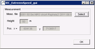
Extreme wind GUI

Extreme-wind estimation at the location of a measurement mast

The tws_file is assumed to contain 10-minute-averaged wind speed data.

$v_50$ value – the extreme wind estimate:

– The 10-minute average wind speed that is reached on average once every 50 years.

Let – $v(t)$ be the wind speed data from the tws_file .

– $R$ be the duration in years of the tws_file, i.e. the time from start to end of the file subtracted

the duration of gaps in the data.

$v_{max,is}$ , maximal values from independent storms:

A list of maximal values from independent storms, $v_{max,is}$ , is extracted from $v(t)$ , where an independent storm is

determined from the 10-hour averaged values of $v(t), v_{10h}(t)$ , and is the maximum of ${v(t_{start}),\dots,v(t_{end})}$ , where $t_{start}$ and $t_{start}$ defines an interval where $v_{10h}(t)$ is continuously above $v_{lull} = 5 \enspace \frac{m}{s}$ , see figure below.

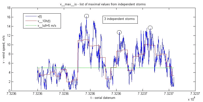
Independent storms

The number of maximal values extracted from v(t) by this method is typically 100 / year.

$v_{max}$ , subset of values from $v_{max,is}$ :

The list of maximal values used in the estimation, $v_{max}$ , is a selection of the highest values in $v_{max,is}$ .

If $v_{max,is}$ is sorted in increasing order, then

$v_{max} = { v_{max,is}(m) , \dots , v_{max,is}(N) }$ ,

where m is the closest integer solution to

${m \over {N+1}^r} = {1 \over 11 }$

Here N is the number of elements in $v_{max,is}$ , $r = N / R$ is the storm rate (events/year).

$v_{50}$

We assume that $v_{max}$ is Gumbel distributed, so the cumulative probability distribution has the form

$F(v) = exp(-exp( -(v - b) / a )$

So that

(1) $v = a(-\ln( -\ln(F(v)))+b = ay+b$

The parameters a and b are determined by weighted least-squares:

Let $y(1) = ln(R) + 0.557$ , and $y(i)=y(i-1)-\frac{1}{i-1}$ , for $i = 2 , \dots , M$ ( # elements in $v_{max}$ ),

and set the variance, $s^2$ , of the i-th sample point according to $s^2(1) = (3.14^2 / 6)-\frac{1}{M+1}$ and

$s^2(i)=(s^2(i-1))^2-\frac{1}{(i-1)^2}$ , for $i = 2 , \dots , M$

We consider v as the independent variable, so that we find the weighted least-squares fit of the line (1)

given the points $(v_{max}(i) ,y(i))$ according to

$y(i) = a'v_{max}(i) + b'$ i=1,\dots,M[/latex], with $a=\frac{1}{a'},\quad b=-b'/a'$ ,

which is the minimum of $S(a',b') = \sum_i w(i)\cdot [y(i)-a'v_{max}(i)-b']^2$ , where the weights are

$w(i) = \frac{1/s^2(i)}{\sum_j ( 1/s^2(j) }$ ( so $\sum_i w(i)=1$ ).

The a’, b’ values minimizing S is found by solving the two equations $dS/da' = 0$ and $dS/db' = 0$ .

The $v_{50}$ estimation is then given by

$v_{50} =[-ln(-ln(0.98))]a + b$

The regression is illustrated in the following figure.

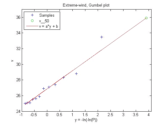
Extreme wind Gumbel plot

Extreme-wind at locations in area close to measurement mast

The $v_{50}$ values at locations x, y and height h above ground are estimated by scaling each measurement entry

in the tws_file according to WindSim simulations of the wind-field – magnitude and direction, and performing

a $v_{50}$ estimation on these scaled tws values.

Assume the measurement mast is located at $x_{tws}, y_{tws}$ , with measurements at height h. Each measurement

is a magnitude, direction pair $v_{tws}, d_{tws}$

Let $v_{ws}(x,y,s)$ and $d_{ws}(x,y,s)$ be WindSim simulations of the wind speed and direction at height h for sectors

$s = 1 , \cdots , 12$ ( 0′ , … , 330′ ) (or the chosen set of sectors)

For each sector s , there is a scale factor for the location x, y, given by

$f(x,y,s) = \frac{v_{ws}(x,y,s)}{{v_{ws}(x_{tws},y_{tws},s)}}$

valid for scaling v_{tws} values in the directions

$d_{ws}(x_{tws},y_{tws},s)$

Let $f(x,y,d)$ be the interpolated value of f for values of d other than $d_{ws}(x_{tws},y_{tws},s), s=1,\cdots,12$

The $v_{50}$ value at location x, y is then estimated:

– Adjust each $v_{tws}$ in the tws file by $v_{tws}(i) = v_{tws}(i) \cdot f(x,y,d_{tws}(i))$

– Perform the $v_50$ estimation on the adjusted $v_{tws}$ values

6.6 Other constraints

Constraints can be added to the Constraints Map by:

Import Shape file (.shp) The shape file can define several polygons.

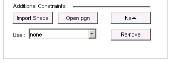
Defining additional constraints

By defining constraints with a drawing editor, pressing New. When a constraint is added with New, it will automatically be saved to the Results Directory, and can later be read with the Open pgn button.

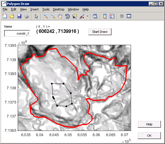
Draw constraints

6. IEC exclusion areas

6. IEC exclusion areas

<<< 2.0.0 Morbi et sodales To overview >>>

6. IEC exclusion areas

6.1 Terrain inclination

6.2 Flow inclination

6.3 Shear

6.4 Turbulence

6.5 Extreme wind

6.6 Other constraints

Search in documentation

Table of contents

Video documentation

Contact

Address

Products

Knowledge