
7. Layout optimization
After the Energy Map and Constraints Map are defined, optimizations of n = 1..N layouts can be performed. The pre-existing constraints of IEC exclusion areas, park areas and other area constraints are already defined in the Constraints Map module. In the layout optimization module, each layout n can be constrained with minimum distance constraints, elliptic distance constraints, effective turbulence constraints, or a combination thereof. The distance constraints are what make layout optimization a difficult problem: where you place one turbine affects where you can place others, due to wake losses and wake-induced turbulence.
7.1 Optimization algorithms
Three alternatives can be selected: Basic Optimizer, WFD cloud optimization and WFD local optimization.
Basic optimization is a heuristic algorithm based on simulated annealing, providing near-optimal solutions. It is the default and requires no extra license.
WFD cloud optimization is a specialized routine based on formal operations research methods, solved by state-of-the-art solvers. It can guarantee global optimum subject to minimum distance, elliptic distance and wake-induced turbulence constraints. It runs as a cloud service (hosted on Google Compute Engine) callable from within ParkOptimizer, purchasable per use or with a periodic license. Requires internet access.
WFD local optimization is the same algorithm deployed as an executable on the client's local server — intended for larger organisations, requiring additional licenses.
7.2 Optimization settings
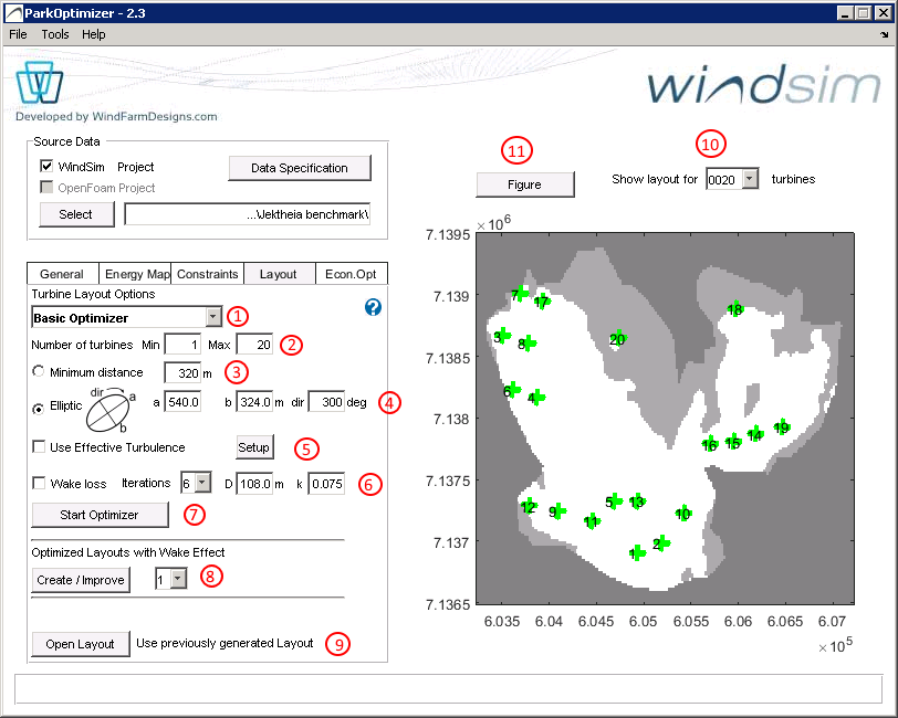
Number of turbines: a special feature of ParkOptimizer is optimizing for a range of layouts n = 1..N — select Min and Max values. Layout size can have a significant impact on profitability and project risk.
Distance constraints: specify either Minimum distance or Elliptic distance with parameters a, b and deg (a = diameter [m] along the major axis, b along the minor axis, deg = orientation of the ellipse major axis). The elliptic distance constraint is a proxy for wake losses and wake-induced turbulence; a typical choice is a = 5 RD, b = 3 RD (RD = rotor diameter), with orientation depending on the wind rose.
7.3 Effective turbulence
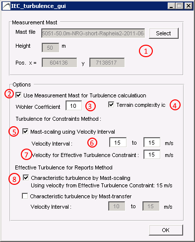
Effective turbulence is specified by checking Use Effective Turbulence and editing the Setup: it is calculated from the .tws mast file (also used in the IEC constraints module), with an option to use a measurement mast, the Wöhler coefficient, and a terrain-complexity index. Characteristic turbulence σ_c should be checked over a range 0.2·V_ref … 0.4·V_ref and should not exceed the 90th percentile of the turbulence standard deviation σ_σ.
7.4 Wake losses
Wake loss calculations are preferably applied after a layout satisfying the minimum distances is created. For wake losses, the N.O. Jensen model is applied:
dV(s) = v₀ · (1 − √(1 − C_t(v₀))) · ( D / (D + 2kx) )²
where x is the downstream distance, D the rotor diameter and k the wake decay coefficient (default 0.075). We recommend not using wake-loss calculations during optimization; run wake adjustments later on a layout where the distance constraints are satisfied. Press Start Optimizer to begin.
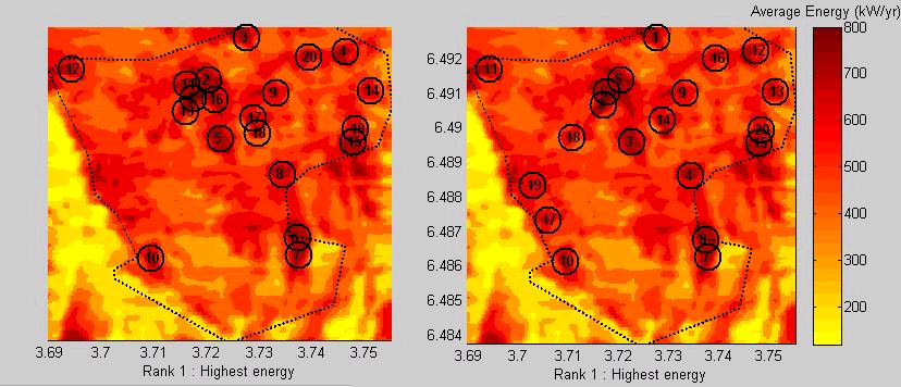
7.5 Improve layouts
Once a layout satisfying the distance constraints exists, run optimized layouts with wake effects; the dropdown defines how many times simulated annealing runs for wake adjustment. Results are written to Results_Directory\OPT_OUT\wake_effect_adjusted. The energy production at each point, incorporating wakes, sums over sectors of ∫ wbl(v, A(s) − dV(s), k(s)) · PC(v) · f(s) dv, used to move turbines so the total energy is higher (Simulated Annealing). All results are stored in OPT_OUT as Layout0001.txt … plus an energy_curve.txt with the corresponding energy yield per layout size.